Master Thesis
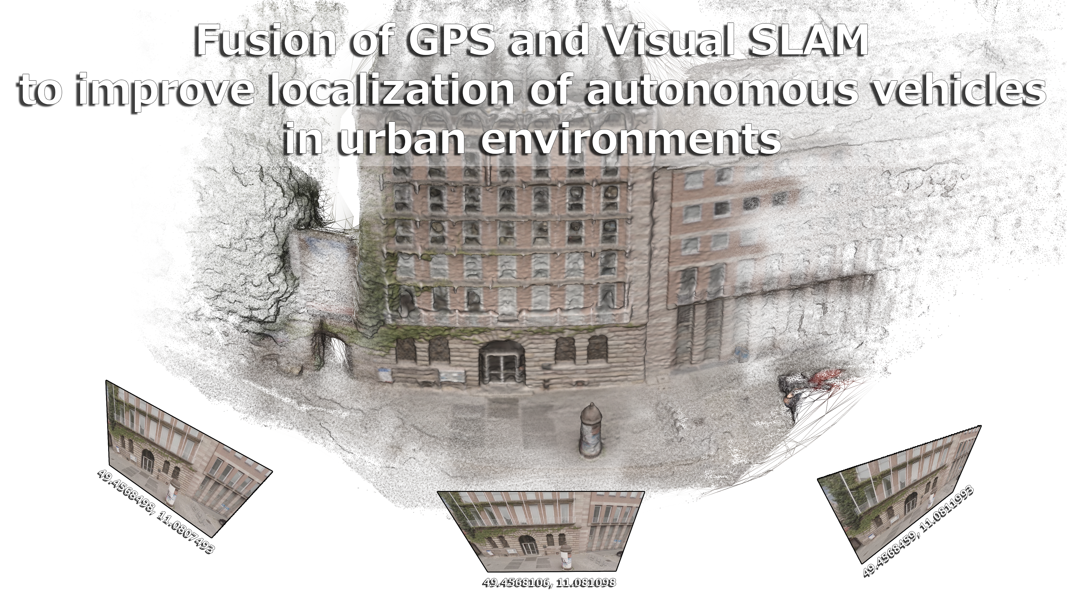
Fusion of GPS and Visual SLAM
to improve localization of autonomous vehicles
in urban environments.
by Adam Kalisz
Agenda
- Last time (Recap)
- This time
- Paper details
- Conclusion / Feeling
Last time
Comparison
Papers VSLAM and GPS Fusion
Variational Methods on
3D reconstruction
This time
Ultra-Tightly Coupled Vision/GNSS
for Automotive Applications
[Aumayer, 2016]
Degree of Doctor of Philosophy (207 pages)
Vision-Aided Pedestrian Navigation
for Challenging GNSS Environments
[Ruotsalainen, 2013]
Degree of Doctor of Science in Technology (181 pages)
Integrating Vision Derived Bearing Measurements with Differential GPS for Vehicle-to-Vehicle Relative Navigation
[Amirloo Abolfathi, 2015]
Degree of Master of Science (135 pages)
sorry, too much :(
but: Some other time!
Today
Open Source 3D Reconstruction from Video
[Mierle, 2008]
Master of Applied Science (124 pages)
1 Introduction
1 Introduction
Motivation:
Increasing number of pictures
Contribution:
Fully open source (!), Blender, Evaluation tool for research
Term "matchmoving":
Used in film industry
1 Introduction
Requirements:
Free, easy, documented, auto-testing, automated
Related work:
Commercial (Boujou, PFTrack, Syntheyes, ...)
and Open (VXL, OpenCV)
Evaluation:
real (range scanning vs. optical flow)
and synthetic (Maya vs. Blender) data sets
2 Reconstruction without the math
2 Reconstruction without the math
Problem:
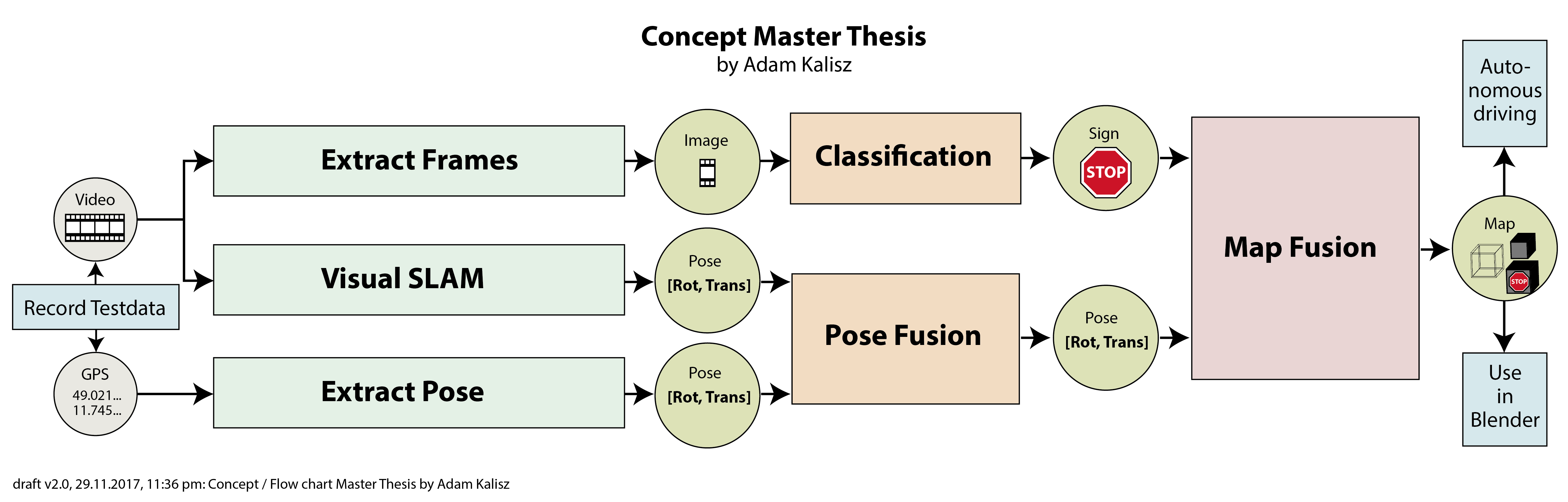
video of a scene -> determine pose of camera and location of some points
Solution:
at highest level see next picture
2 Reconstruction without the math
2 Reconstruction without the math
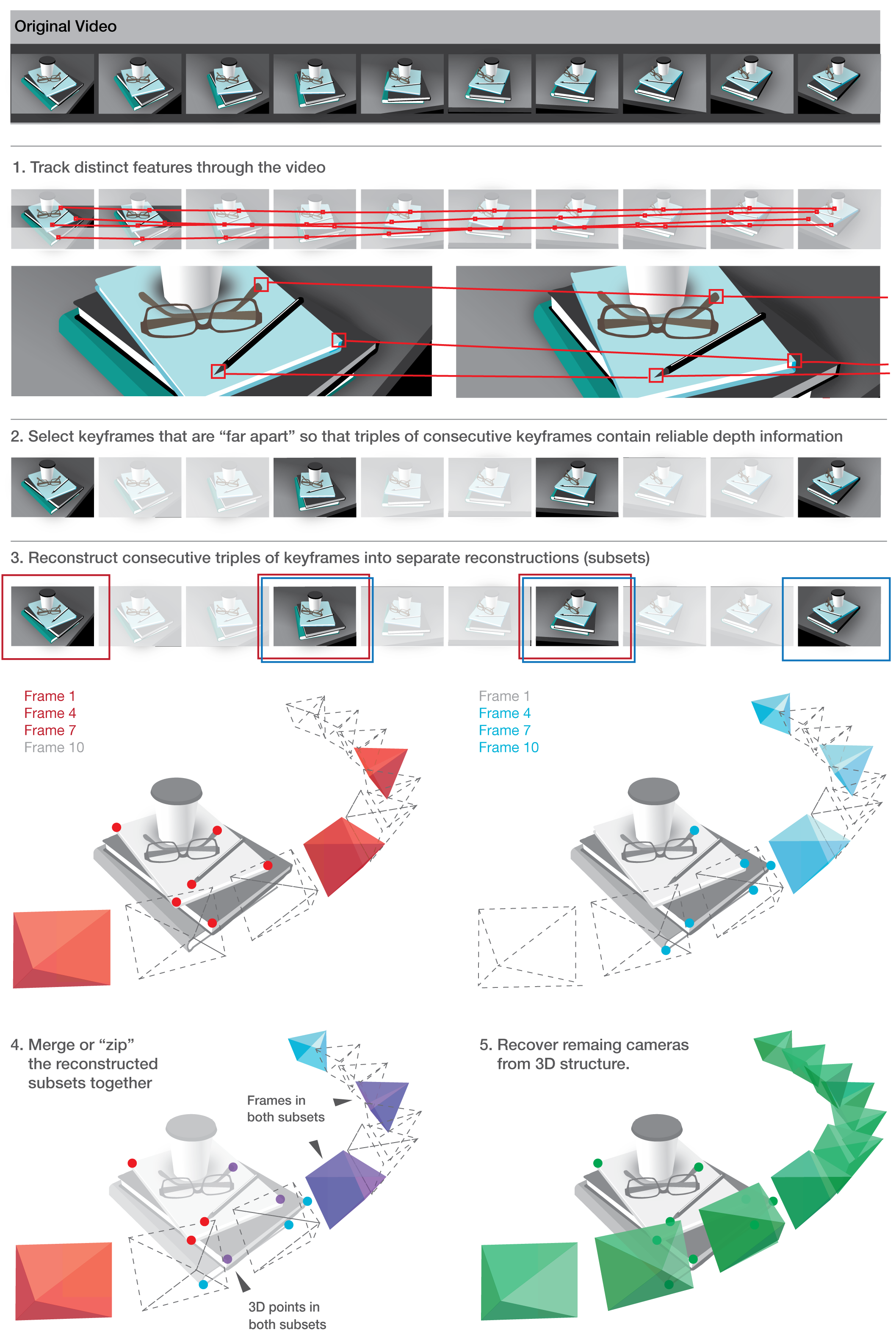
Find "good" features (2D)
Track features across frames (2D)
Discussion: Points vs. lines or curves or planes
No clear "best" strategy to recover
cameras and structure
2 Reconstruction without the math
Closed-form-solutions

2 Reconstruction without the math
Closed-form-solutions
- (A) 7 * 2D-2D [=cams+points]
- (B) 6 * 2D-2D-2D [=cams+points]
- (C) 6 * 2D-2D-2D-2D [=cams+points]
- (D) 6 * 2D-3D (camera resectioning) [=1 cam]
- (E) 1 * 2D-2D (triangulation) [=1 point]
If perfect data: Use (B) then (D).
But...!
2 Reconstruction without the math
I) Tracks are unreliable: Outliers and drift
-> Solution: robust fitting (e.g. RANSAC)
-> Example: randomly pick six correspondences and try to solve for closed-form (compare 6 * 2D-2D-2D). Increase score of track if reprojection of 3D points into camera is close. Repeat to find best score.
2 Reconstruction without the math
II) Tracks are short: no longer than a few seconds
-> Solution: Merge multiple "triplets" of tracks into one
-> Pollefeys et al. (2004): Grow tracks by alternating closed-form-solutions
2 Reconstruction without the math
Critical issues:
- I) Insufficient camera motion between frames
-> Widen the baseline: Choose (key-)frames with strong depth - II) Camera calibration (focal length, aspect ratio, and principal point)
-> Autocalibration always worse than manual calibration - III) Barrels, pincushions, and Fisheyes
-> undistort lens or run bundle adjustment
3 The reconstruction system
3 The reconstruction system
For end user: Set of command line tools (9 to 10 steps)
$ mplayer -vo pnm:pgm video.avi
$ track sequence --pattern="%08d.pgm" --output="video.ts.json" --num features=500 --start=1 --end=100
$ correct radial distortion --track="video.ts.json" --output="video corrected.ts.json" --intrinsics="CanonSD500.k.json"
$ pick keyframes --track="video corrected.json" --output="video.kf.json"
$ reconstruct subsets --track="video corrected.json" --bundle subsets=true --keyframes file="video.kf.json" --output="video.prs.json" --ransac rounds=100
$ merge subsets --track="video corrected.json" --subsets="video.prs.json" --output="video.pr.json" --bundle subsets=true
$ resection --track="video corrected.json" --reconstruction="video.prs.json" --output="video resectioned.pr.json" --bundle subsets=true
$ metric upgrade --track="video corrected.json" --reconstruction="video resectioned.prs.json" --intrinsics="CanonSD500.k.json" --output="video.mr.json"
$ export blender --track="video corrected.json" --metric reconstruction="video.mr.json"
--intrinsics="CanonSD500.k.json" --output="video.py"
3 The reconstruction system
Preliminaries
Projective Geometry
It's really just homogeneous coordinates
Points at infinity (line intersection)
Represent all points from ${\rm I\!R}^3$ as projection in ${\rm I\!R}^2$
(up to a scale factor)
=> $[4x; 4y; 4]^T$ is the same as $[x; y; 1]^T$, (0 is infinity)
3 The reconstruction system
Camera Projection Model
Standard Euclidean projection
$\begin{align} \begin{bmatrix} x \\ y \\ z \end{bmatrix} \end{align}$ = $K[R(\hat{X}-C)]$, $\begin{align} \begin{bmatrix} \hat{x} \\ \hat{y} \end{bmatrix} \end{align}$ = $\begin{align} \begin{bmatrix} x / z \\ y / z \end{bmatrix} \end{align}$
translate, rotate 3D Points $\hat{X}$
scale by intrinsics Matrix K
3 The reconstruction system
Camera intrinsics
$\begin{align} K &= \begin{bmatrix} focal_x && skew && center_x\\ 0 && focal_y && center_y \\ 0 && 0 && 1 \end{bmatrix} \end{align}$
Without zooming, K is fixed for all images.
3 The reconstruction system
Lens distortion
$x^{''} = x^{'}(1 + k_1 r^2 + k_2 r^4) + 2p_1x^{'}y^{'} + p_2(r^2 + 2x^{'2})$
$y^{''} = y^{'}(1 + k_1 r^2 + k_2 r^4) + 2p_2x^{'}y^{'} + p_1(r^2 + 2y^{'2})$
$(r^2 = x^{'2} + y^{'2})$
Normalized image coords: $x^{'}$, $y^{'}$
radial distortion $k_{1,2}$
tangential distortion $p_{1,2}$
Perspective division -> distortion -> intrinsics
3 The reconstruction system
Kanade-Lucas-Tomasi (KLT) tracker
- 1.) Find outstanding features to track (extra talk!)
- 2.) Track features across sequence
KLT more efficient way to minimize:
$\epsilon(\textbf{d}) = \frac{1}{2} \int\int_{Windows}^{} [J(\textbf{x} + \textbf{d}) - I(\textbf{x})]^2 weight(\textbf{x}) d\textbf{x} $
$I(\cdot)$ gray value frame1, $J(\cdot)$ gray value frame2, $\textbf{x}$ feature in frame1, $\textbf{d}$ displacement
Cross-Correlation-Search: Extremly slow!
3 The reconstruction system
Kanade-Lucas-Tomasi (KLT) tracker
uses Taylor expansion to reduce problem
Task left: Solve a 2x2 linear system
3 The reconstruction system
Radial unwarping
When camera calibration information is available:
- I) unwarp the video before tracking
(using a Levenberg-Marquardt minimizer) - II) or: unwarp the correspondences after tracking
If not:
incorporate distortion terms
into the final bundle adjustment
(Calibration was not part of libMV, instead OpenCV was used)
3 The reconstruction system
Keyframe selection
Two metrics used by libMV:
- count the number of tracks that survive from a reference frame
- use a bucketing procedure in which the track count is constrained to image blocks
3 The reconstruction system
Subset reconstruction
three-frame six-point closed form solution described by Schaffalitzky et al. [2000].
fails miserably if one of the six points is in error ("outlier")
3 The reconstruction system
therefore use closed form solution as a RANSAC driver
- Randomly choose a subset of 6 points from correspondences ("inliers")
- Fit this subset using the three-view six-point algorithm
- Score the projective reconstruction and compare how well it matches rest of the data
- Repeat 1.) and 2.) until probability of good set of points is found
3 The reconstruction system
Calculating residual errors
- Triangulate 2D point position from images 1 and 3 to get 3D point
- Project 3D point into image 2
- residual error is the difference between reprojected image location and tracked (measured) image location
3 The reconstruction system
Scoring methods:
many to choose from
- RANSAC
- LMedS
- MSAC
- AMLESAC
- MLESAC (mixture model of 2D Gaussians)
- AMLESAC2 (mixture of Rayleigh distributions, used in libMV)
3 The reconstruction system
Residual error
Assuming tracked points have isotropic additive Gaussian noise, Rayleigh distribution is a good model of the magnitude of reprojection errors.
$p(x; \sigma_i, \sigma_o, \gamma) = \gamma p(x; \sigma_i) + (1 - \gamma) p (x; \sigma_o)$
$x$=magnitude of residual error, $\sigma_i$ variance of inliers, $\sigma_o$ variance of outliers, $\gamma$ inlier fraction
AMLESAC2 fits above simultaneously via Expectation Maximization, scores on inlier variance
3 The reconstruction system
Bundle adjustment
after coarse reconstruction from closed-form solutions, adjust all the reconstruction parameters simultaneously to minimize reprojection error
=> nothing more than nonlinear minimization
Many details which will be skipped here, can be a separate talk.
Mostly continues with intelligent way to penalize errors
This is an important step for reconstruction.
3 The reconstruction system
Merging subsets
libMV implements the one-frame overlap method
(one camera in common)
in Practice, merging projective reconstructions is quite unreliable.
Hence, score subsets of 2 points from set of 3D correspondences and test repeatedly.
3 The reconstruction system
Merging subsets
Again, LMedS, RANSAC, MLESAC, etc. are used
Nonlinear refinement is done using Levenberg-Marquardt
Hierarchical merging (binary tree upwards) as opposed to sequential for errors not to accumulate at the end of the reconstruction
3 The reconstruction system
Resectioning
Recover remaining cameras to complete reconstruction
Each correspondence produces two equations expressed as a matrix
Compute missing camera matrix via SVD
Use RANSAC again to remove outliers
3 The reconstruction system
Metric upgrade
"Projective reconstruction" is superset
of "Euclidean (metric) reconstruction"
Projective camera: $(K,R, \textbf(t))$
Euclidean camera: $P = K[R|\textbf(t)]$
(homogeneous matrix)
3 The reconstruction system
Metric upgrade
Goal: Find upgrading transformation ($H$) from projective reconstruction ($P$) and camera intrinsics ($K$).
Not supported back then: autocalibration (included now).
3 The reconstruction system
Metric bundle adjustment
Metric upgrade produces bad quality
Reason: rotation components of camera matrices were forced to be orthogonal
Effect: Drastically changes the projected image coordinates
Solution: Bundle adjustment (same as projective BA, but using euler angles)
3 The reconstruction system
Point cloud alignment for evaluation
Evaluation with ground truth is hard, because of translation, scale, and rotation ambiguity (similarity transform)
Example: Photo of car against white background -> is this a real car or a 10cm model?
3 The reconstruction system
Point cloud alignment for evaluation
Solution: Scale and align with ground truth data
- Subtract the mean from both point clouds
- Divide each point cloud by mean distance from origin
- Orthogonal procrustes (use SVD):
$\min\limits_{R} = || A_{3xN} - RB_{3xN} ||^2$ - Combine into a single 4x4 transformation matrix
4 Evaluation of Multiview Algorithms
Synthetic: Point cloud from 3D scene, projected into image space, perturbed
Autocalibration: Final reconstruction more important to evaluate than recovered intrinsics (in practice)
Rendered images: Advantages like ground truth and control parameters (exposure, noise, distortion)
Blender community helped to provide renderings for evaluation
5 Results
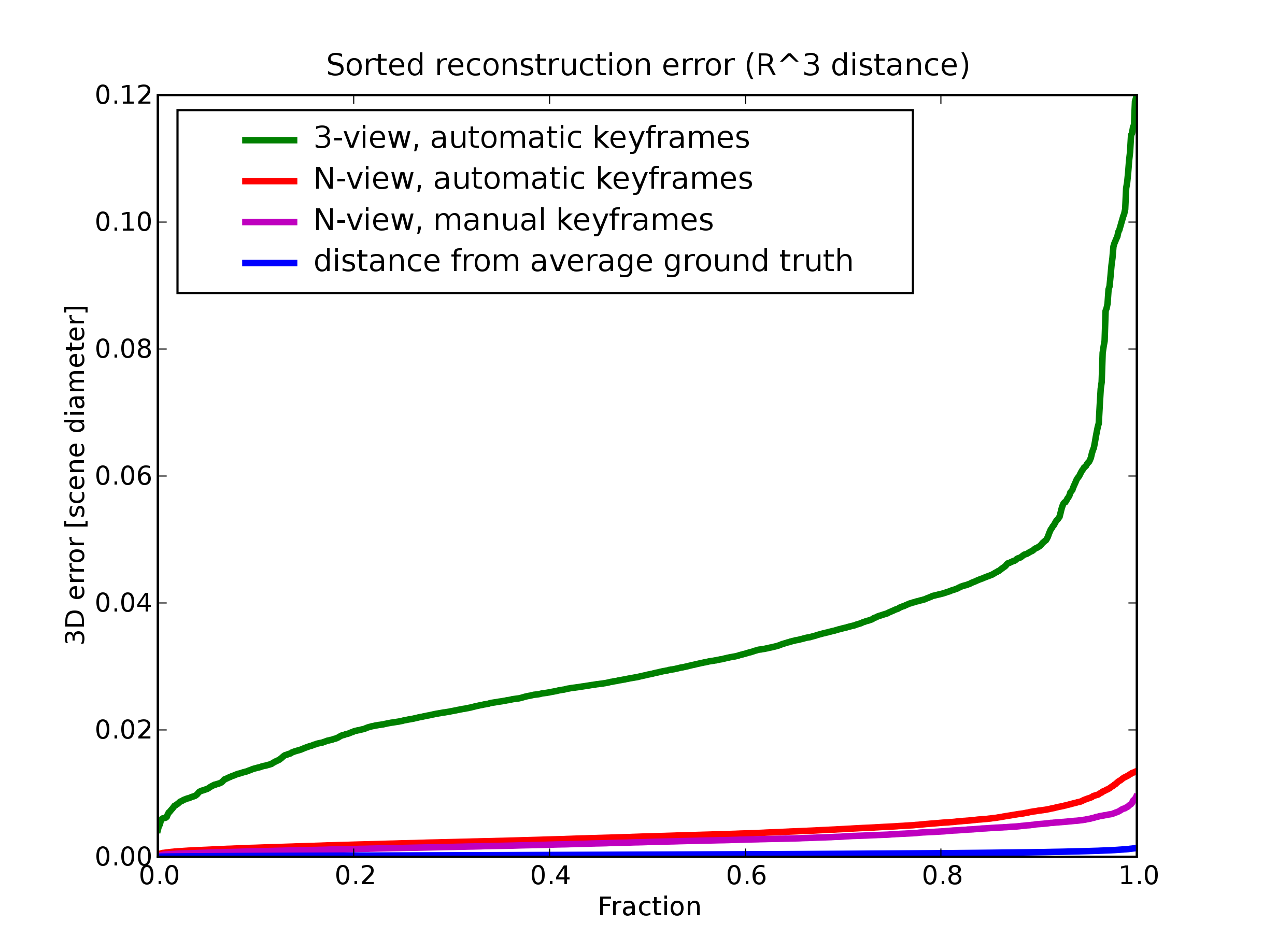
N-view instead of 3-view reconstruction gives better results
Manual selection of keyframes gives better results than automatic selection
Conclusion
- a long read (124 pages)
- but a good one!
Pressure is growing!
Feeling